Decoding pan-cancer treatment outcomes using multimodal real-world data and explainable artificial intelligence

Cohort definition

We retrospectively evaluated data from 150,079 patients with cancer with available medical records treated at the West German Cancer Center of the University Hospital Essen, one of Germany’s largest academic comprehensive cancer centers. Of these, 15,726 patients (44.3% female) who received systemic cancer treatment between April 2007 and July 2022 (median: November 2016) were included in the final analysis (Extended Data Fig. 1). The most frequent cancer entities were lung cancer (n = 4,320), sarcoma (n = 1,578) and breast cancer (n = 1,223; for details, see Supplemental Table 1). Censoring was performed on 7,349 patients (46.7%) to calculate overall survival (OS) and on 5,638 patients (35.9%) to calculate time to next treatment (TTNT). Metastatic status (M status) was available in a structured format at baseline for 7,965 patients. Of those, 5,606 patients were treated for metastatic disease (M1), and 2,359 patients received systemic therapy for localized or locally advanced cancers (M0). In 5,395 patients, body composition was automatically assessed from abdominal CT images taken before treatment initiation^23,24. In total, we included 350 variables in our analysis, consisting of different modalities and both patient- and tumor-specific variables, providing a detailed patient characterization before the first systemic treatment at our institute (Fig. 1).

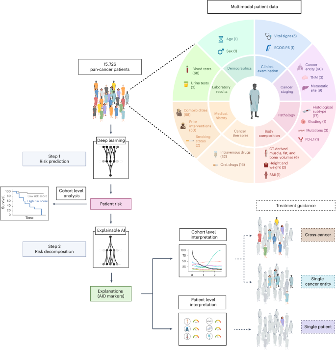
Following the collection of multimodal pan-cancer data, each patient’s risk score is predicted by deep learning and enables patient stratification. xAI then decomposes the patient risk into the individual contributions of each marker. This enables treatment guidance at the patient and cohort level. The numbers in parentheses indicate the number of variables for each data type.

Development of pan-cancer models for outcome prediction

Two neural networks were trained to predict OS or TTNT for each patient based on their medical profile at the time of first in-house systemic treatment. We demonstrated the reliability of the neural networks by performing a five-fold cross-validation for OS and TTNT prediction, respectively. For each fold, 80% of the data were used for training the neural network, 10% for hyperparameter tuning and 10% for testing. Calibration results are shown in Extended Data Fig. 2.

The survival model achieved an average concordance index (C-index) on the pan-cancer dataset of 0.762 (range across folds: 0.758–0.764) for OS prediction and 0.711 (range: 0.702–0.718) for TTNT prediction of patients across all cancer entities (Fig. 2a). When the model performance was tested independently for each cancer entity with at least 20 patients in each fold’s test set, the predictive performance varied. For OS, the highest C-index was achieved for ocular cancers (0.804, range: 0.771–0.860), whereas the highest C-index of TTNT was achieved for rectal cancers (0.756, range: 0.644–0.800).

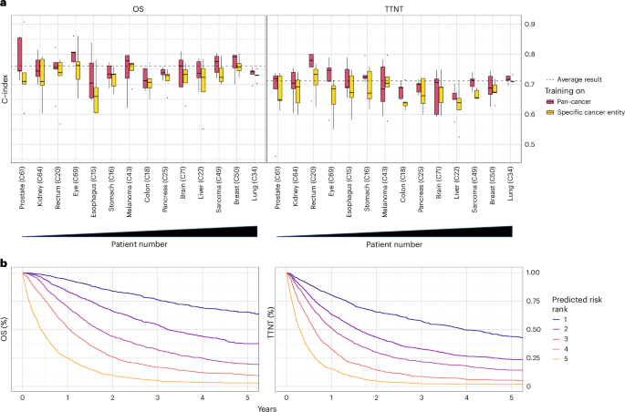
a, Concordance index for predicting OS and TTNT in five-fold cross-validation. The dashed line indicates the prediction result over all patients averaged across folds. Box plots show prediction results for individual cancer entities with at least 20 patients in the test set (n = 6,070 patients overall; prostate: n = 131; kidney: n = 147; eye: n = 187; esophagus: n = 198; rectum: n = 199; stomach: n = 300; pancreas: n = 304; brain: n = 312; colon: n = 319; melanoma: n = 324; liver: n = 373; sarcoma: n = 538; breast: n = 619; lung: n = 2,119) of each fold after training the neural network on all cancer entities (red) or the specific cancer entity (yellow). Cancer entities are ordered from left to right by ascending patient numbers in the overall dataset. Median is indicated by center line, bounds of boxes indicate interquartile range, and whiskers extend to a maximum distance of 1.5 ⋅ IQR from the hinge. Data beyond the end of whiskers are plotted individually. b, Kaplan-Meier plots for OS and TTNT in the pan-cancer dataset for patients of the combined test sets (n = 7,861) patients. Patients were stratified into five risk groups according to the risk predicted by the (pan-cancer trained) neural network.

Source data

Training models on the pan-cancer dataset, as opposed to exclusively training on single cancer entities, significantly improved model performance for both OS (mean C-index of patients within individual cancer entities: 0.75 versus 0.72, P < 0.001) and TTNT (mean C-index of patients within individual cancer entities: 0.70 versus 0.68, P < 0.001). Only in melanoma patients, the mean results (mean C-index for OS: 0.74 versus 0.75, mean C-index for TTNT: 0.69 versus 0.7, P > 0.05) were better when the training was performed on the melanoma cohort compared to training on the pan-cancer cohort. The advantage of the pan-cancer model over the single-entity models suggests that it used prognostic information shared by the overall cohort to provide robust predictions.

After training on a large and granular real-world pan-cancer dataset, both neural networks for predicting OS and TTNT were able to stratify patients from the test sets into distinct cross-cancer risk groups (Fig. 2b).

We compared the performance of the pan-cancer models against common prognostic scores (Fig. 3a–h). Reporting the average C-index, the xAI model outperformed UICC Staging (OS: 0.75 versus 0.56, P < 0.001; TTNT: 0.70 versus 0.54, P < 0.001), the Eastern Cooperative Oncology Group Performance Status (ECOG PS; OS: 0.81 versus 0.67, P < 0.001, TTNT: 0.72 versus 0.62, P = 0.001), the Charlson Comorbidity Index (CCI, OS: 0.75 versus 0.63, P < 0.001, TTNT: 0.69 versus 0.61, P < 0.001) and the modified Glasgow prognostic score (mGPS, OS: 0.76 versus 0.59, P < 0.001, TTNT: 0.70 versus 0.56, P < 0.001).

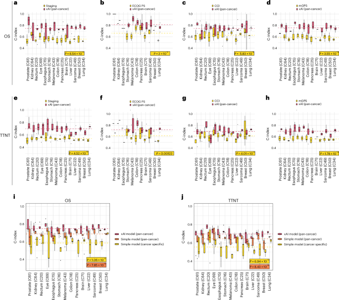
a–h, Filtered for patients for whom clinical markers were present. Lines indicate the average of all C-indices calculated for each fold and cancer type. a,e, UICC Staging (n = 7,572 patients, P = 6.54 × 10⁻¹¹ and 4.52 × 10⁻¹²). b,f, Eastern Cooperative Oncology Group performance status (ECOG PS) (n = 2,035 patients, P = 2 × 10⁻⁵ and 0.00122). c,g, Charlson Comorbidity Index (CCI; n = 7,965 patients, P = 5.83 × 10⁻⁹ and 4.01 × 10⁻⁶). d,h, Modified Glasgow prognostic score (mGPS; n = 6,042 patients, P = 3.55 × 10⁻¹⁴ and 1.78 × 10⁻¹⁴). i,j, Comparison between the pan-cancer xAI model and a parsimonious Cox model trained on all patients or on patients with the test set tumor type for OS (i, n = 6,070 patients, P = 1.06 × 10⁻¹² and 7.85 × 10⁻¹²) and TTNT (j, n = 6,070 patients, P = 6.94 × 10⁻¹³ and 8.43 × 10⁻¹²). Median is indicated by center line, bounds of boxes indicate interquartile range and whiskers extend to a maximum distance of 1.5 ⋅ IQR from the hinge. Data beyond the end of whiskers are plotted individually. P values are derived from Wilcoxon ranked test (two sided).

Source data

For clinical deployment, a small set of variables would facilitate the application of models. Therefore, we compared the xAI model to a simplified Cox model fitted on ten automatically selected variables (Fig. 3i,j). The pan-cancer xAI model outperformed the simplified model when fitted on the complete training dataset (average C-index: 0.75 versus 0.69, P < 0.001) and when fitted on the respective cancer type (average C-index: 0.75 versus 0.59, P < 0.001).

xAI reveals complex prognostic relationships between markers

After developing reliable outcome prediction models, we applied xAI to unravel how clinical information of individual patients influences the neural networks in assessing prognosis. We chose to explain the pan-cancer models since they outperformed cancer-specific models overall. We selected the xAI method layer-wise relevance propagation (LRP) because it allows for the computation of robust explanations at low computational cost for individual patients¹². LRP computed for each patient the risk contribution (RC) of every clinical variable, such as laboratory markers or comorbidities, to the predicted favorable or unfavorable outcome. This results in AI-derived (AID) markers with two dimensions, the original marker value and its LRP-assigned RC. A positive RC indicates a contribution to an adverse outcome and a negative RC indicates a contribution to a favorable outcome.

By analyzing the AID markers across all patients, it was possible to investigate how the neural network evaluated the relationship between the marker and its contribution to the patient’s risk (Fig. 4a). For example, increasing age and elevated levels of C-reactive protein (CRP) strongly contributed to predicting an unfavorable prognosis. In contrast, high fT3, high PD-L1 TPS and higher CT-derived abdominal muscle volume contributed to predicting a favorable prognosis.

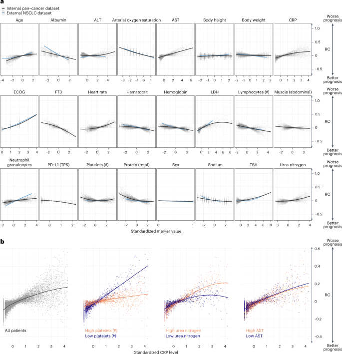
a, Marker RC on the OS prediction. Each point represents one marker value for one patient versus the LRP-assigned RC (y axis) to the patient’s prognosis. Marker values are standardized. b, RC of CRP depended on the value of other markers. The left plot shows the standardized CRP level and LRP-assigned RC for all patients. The right three plots depict the patients for whom the three selected markers: platelet count, urea nitrogen and AST, were in the highest or lowest 10% quantile.

Source data

We validated the results for a subset of markers using external data from 3,288 patients with non-small cell lung cancer (NSCLC) provided by Flatiron Health. Upon applying our approach to the external dataset, we found a strong correlation between the linearized slopes of RCs on the internal and external datasets (Pearson’s r = 0.9, P < 0.001; Extended Data Fig. 3a). Thus, xAI predicted a comparable impact of markers on patient risk in both datasets. To confirm if the fundamental results of LRP matched conventional models, we examined the simplified linearized effect predicted by xAI against a standard Cox proportional hazards model. Our analysis revealed that the relationships computed on the internal and external datasets strongly correlated to the hazard ratios of each marker (subset of markers measured in both datasets: internal dataset: Pearson’s r = 0.93, P < 0.001, external dataset: Pearson’s r = 0.97, P < 0.001, Extended Data Fig. 3b,c; all markers in internal dataset: Pearson’s r = 0.85, P < 0.001, Extended Data Fig. 3d).

Notably, the RC of a marker varied widely even when different patients had the same marker value. By utilizing LRP, it becomes possible to explain some of the variance in RC by marker interactions (Fig. 4b). We observed how the RC of CRP varied depending on the values of additional ‘secondary’ variables. Out of 8,294 examined marker pairs, 1,373 (16.6%) showed significant interactions according to a mixed-effects model. For example, high CRP levels were assigned a high RC, particularly when platelet counts were low (Δ RC slopes: ×0.07, P < 0.001). CRP had less influence on the predicted risk when the platelet count was high. Although the prognostic significance of elevated CRP levels and platelet counts is known, the exact interaction has not yet been described²⁵. The impact of blood urea nitrogen (BUN) on the RC of CRP was less pronounced (Δ RC slopes: 0.03, P < 0.001). Here, a higher CRP level was associated with a particularly high RC in patients with high BUN levels. In contrast, the RC of CRP was independent of aspartate aminotransferase (AST) (Δ RC slopes: −0.006, P = 1.0).

The statistically significant interactions between the variables present in the internal and external datasets showed a high level of similarity in the external dataset (Pearson’s r = 0.59, P = 0.021; Extended Data Fig. 3e). To confirm that the fundamental interaction results observed with xAI were consistent with conventional models, we examined the simplified linearized effect over the LRP-assigned RC against a mixed-effects Cox proportional hazards model.

Here, the direction of interactions derived from xAI matched the interactions observed with the Cox regression models in the internal and external datasets (r = 0.91, P = 0.03 and r = 0.69, P = 0.009; Extended Data Fig. 3f,g). Based on these results, we concluded that the LRP approach was highly reproducible across various datasets as well as consistent with established statistical models that simplify relationships. However, the xAI approach’s full potential extends beyond this and enables nonlinear RC assignments for individual patients, taking into account their unique disease context.

For results on TTNT, see Extended Data Figure 4a,b.

AID markers for patient-level treatment guidance

AID markers, the combination of a marker value with its LRP-assigned RC, enhance the clinical information available to healthcare professionals by incorporating the contextual risk associated with each marker. A ‘clinician’s guide’ can clearly present the AID marker profile of individual patients.

In Fig. 5, we show representative results that illustrate a potential real-world use case of the ‘clinician’s guide’ for four different patients. In patient 1, age, BMI, body weight, and fT3 values contributed unfavorably to the overall prognosis, while the high lymphocyte and platelet counts were assigned a favorable (negative) RC. The patient’s prognosis deteriorated with impaired breathing, aphagia, pain and an advanced T and M stage. Among the different distant metastases, liver metastases were identified as particularly unfavorable compared to lung and bone metastases. Overall, the neural network therefore predicted a highly adverse outcome for this patient based on all available data. In patient 2, lymphocytopenia and older age particularly contributed to a poor prognosis. However, this patient had few comorbidities, with pleural effusion having the strongest unfavorable impact. The absence of liver metastases and the treatment with pembrolizumab were assigned a favorable RC, and the overall risk was considered intermediate. Notably, patient 3 had elevated CRP levels, which is conventionally associated with a potentially dangerous patient condition requiring increased monitoring. However, xAI does not consider this variable to be detrimental in this particular case, possibly because of this patient’s high platelet count and low urea nitrogen levels (Fig. 4). Patient 4 showed medium visceral adipose tissue (VAT), contributing favorably, and low subcutaneous adipose tissue (SAT), contributing adversely. With few comorbidities and no metastases, the overall prognosis was favorable.

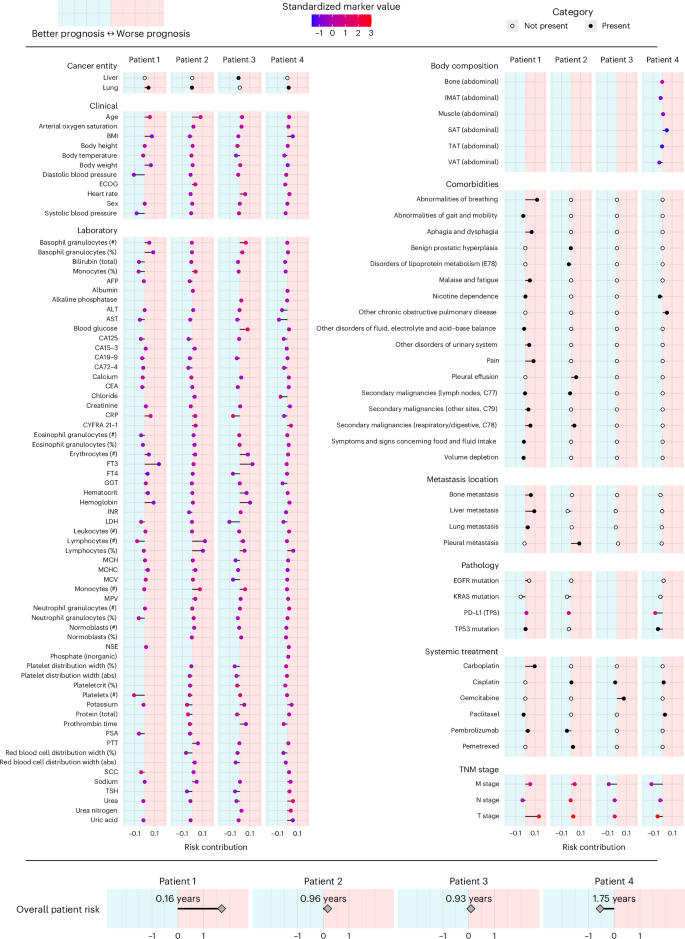
Representative results of four patients are presented. The x axis indicates the marker’s RC toward higher (right/positive) or lower (left/negative) risk. Colors indicate the presence (black) or absence (white) of cancer entities, comorbidities, metastasis locations and systemic treatment. For markers with ordinal or continuous scales, the point color indicates the marker value for the respective patient. For continuous markers, marker values are standardized. The predicted overall patient risk is displayed at the bottom. To facilitate interpretation, the median absolute survival of 100 patients with a similar predicted risk is given. Body composition markers: abdominal volumes of visceral adipose tissue (VAT), total adipose tissue (TAT), subcutaneous adipose tissue (SAT), intermuscular adipose tissue (IMAT), muscle, bone.

Source data

Evaluation of established scoring systems

Our results illustrated the limitations of single marker-based outcome prediction and emphasized the importance of prognostic variables to be considered in the disease context characterized by other markers. In clinical routine, however, it is common to rely on a few scoring systems, such as the TNM stage, to assess prognosis and guide treatment. Based on these scoring systems, patients are usually rigidly categorized, regardless of fundamental differences such as sex, nutritional status or comorbidities.

To evaluate the dependency of a score on this disease context, we analyzed the correlation between the score and the LRP-assigned RC (Extended Data Fig. 4c). For Eastern Cooperative Oncology Group performance status (ECOG PS) (r = 0.87), M stage (r = 0.92), and N stage (r = 0.76), higher scores correlated with higher computed RC on average, indicating a consistent influence on the prognosis independent of other markers. The weak correlation of tumor grade (r = 0.02) and T stage (r = 0.07) with their RC suggested that they should be interpreted in the context of additional markers.

Assessment of marker importance at the cohort level

In a multimodal real-world dataset reflecting clinical care, there are expected to be both sideline markers of low prognostic relevance and critical markers that are highly relevant across patients. To measure the marker importance (MI) in a cohort, we calculated the absolute value of the RC in consistency with other methods in the field¹³. We found that 90% of LRP scores were assigned to the 114 most important markers out of 350 (Extended Data Fig. 5a,b). Across all patients, the most important markers for the prediction of OS were C-reactive protein level (CRP, mean MI: 0.071), free triiodothyronine (fT3, mean MI: 0.066), ECOG PS (mean MI: 0.061), M stage (mean MI: 0.058) and LDH (mean MI: 0.055; Extended Data Fig. 6a,b). These results are consistent with previously reported findings^26,27,28,29. However, our results suggest that fT3 may play a more important role in prognostic assessment than is currently recognized in clinical practice.

Events that are rare in certain cancer subgroups may be common enough in the pan-cancer dataset for models to assess the prognostic impact of the variable. LRP can assess the influence of comorbidities, defined by ICD codes, and medical interventions, defined by the German operation and procedure classification system (OPS), in the disease context (Extended Data Fig. 6c,d). Due to the scarcity of each comorbidity, MI was not informative here, which is why we report the mean RC of affected patients. We found that the comorbidities that contributed the most to the prediction of a poor outcome were pain (mean RC: 0.064), respiratory abnormalities (mean RC: 0.064), ascites (mean RC: 0.056), secondary malignant neoplasm of the respiratory or digestive tract (mean RC: 0.048) and pleural effusion (mean RC: 0.046). Notably, some diagnoses contributed favorably to the overall prognosis (for example, heart failure, gastritis and duodenitis). The interventions that were assigned the highest RC were ureteral stenting (mean RC: 0.074), which may indicate a stenotic process, and meningeal reconstruction (RC: 0.049).

Cross-cohort comparison of prognostic markers

Model training on a pan-cancer dataset and sample-wise explanations obtained by LRP allowed us to investigate how the MI of a marker differed between patient subgroups (Fig. 6).

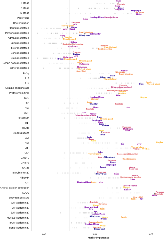
The x axis shows the MI on a logarithmic scale. The three cancer entities with the highest marker MI are annotated for each marker. Body composition markers: Abdominal volumes of VAT, TAT, SAT, intermuscular adipose tissue (IMAT), muscle, bone. Cancer entities are shown only if the respective marker has been measured in at least 20 patients.

Source data

Expectedly, LRP identified many markers whose significance in prognosticating a particular cancer type is already established: CA19-9 had the highest MI in cancers of the small intestine, and biliary tract and bilirubin emerged as an essential marker for liver, pancreatic and biliary tract cancers^30,31,32. The presence of liver metastases was most relevant for cancers of the thyroid gland, rectosigmoid junction and additional digestive tract cancers^33,34. HbA1c was most important in cancers of the pancreas and liver^35,36. The tumor marker CEA had the highest MI in cancers of the rectosigmoid junction, colon and thyroid^37,38.

However, the cross-cancer approach also made it possible to identify many previously unexplored prognostic associations. Abdominal muscle volume, as determined by CT-based body composition analysis, was most important for vulvar, uterine and testicular cancers. Interestingly, AST had very high MI for urethral cancer, followed by the expected high MI for liver and ocular cancer (mainly uveal melanoma). Alanine transaminase appeared to be most important for the prognostic stratification of patients with cancers of the vulva and ovary. The ECOG PS was particularly important for pancreatic, prostate and liver cancers. Apart from thyroid cancer and brain cancers for which this relationship is well known, fT3 was most important in testicular cancer^39,40.

For results on TTNT, see Extended Data Fig. 7.

Evolution of marker importance during disease progression

Having examined the cancer entity-specific impact of markers on prognosis, we further explored their varying importance for prognostication during disease progression. Ordering the deceased patients according to OS, we could follow the LRP-assigned marker importance along a pseudo timeline and observed distinct changes over the course of treatment (Fig. 7). ECOG PS and CRP and LDH levels were highly prognostic markers throughout disease progression across all cancer entities. The prognosis of patients with a short OS was strongly influenced by total serum protein concentration, which may reflect the relevance of organ dysfunction at this stage of the disease, particularly of the liver and kidneys. The coagulation variable prothrombin time and oxygen saturation were highly prognostic in patients with short OS but contributed much less to the prognosis of patients with long OS. M stage had an overall decisive marker importance, which decreased for disease stages with short OS.

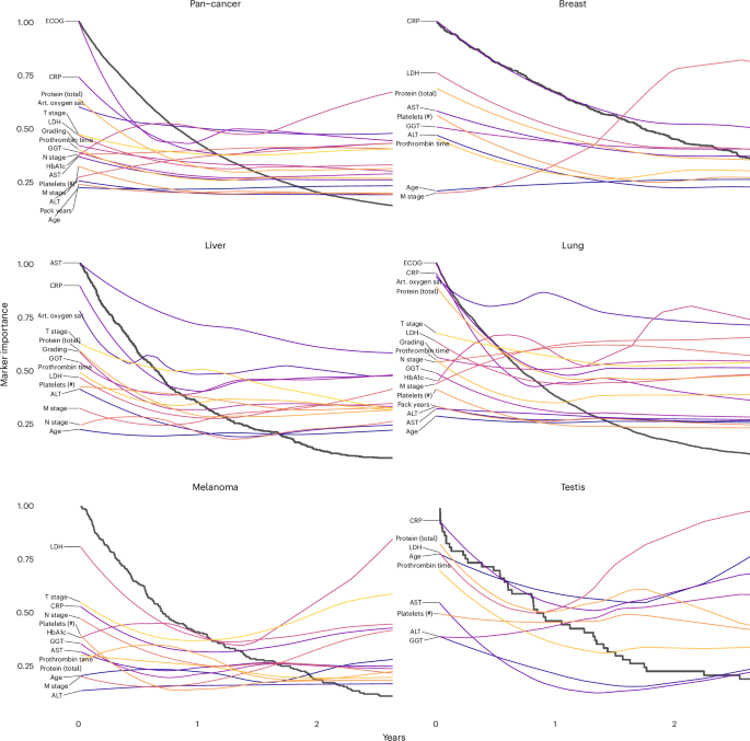
Black lines represent Kaplan-Meier plots, whereas the colored lines visualize the change in marker importance (MI) for patients with different survival times. MI lines are scaled between zero and one. Only deceased patients were included in this analysis (pan-cancer: n = 8,377, breast: n = 487, liver: n = 451, lung: n = 2,753, melanoma: n = 206, testis: n = 50). Selected markers were measured in at least 40 patients and within a 2-year window. Art. oxygen sat., arterial oxygen saturation.

Source data

Our modular approach allowed us to generate explainable Kaplan-Meier plots of patient subgroups with different prognoses. In lung cancer, arterial oxygen saturation had the highest MI for most patients, but for patients with short survival, protein expression, CRP and ECOG PS became even more critical. Metastasis (M stage) generally had higher MI than lymph node metastasis and tumor stage. Interestingly, the importance of metastasis decreased during disease progression and was overtaken by T stage and N stage in patients who survived only a few months. LDH had exceptionally high MI in testicular cancer and melanoma, which is well known in the literature^41,42. The MI of the latter increased during disease progression. In the liver, the MI of AST, total protein, GGT, prothrombin time and LDH increased during disease progression. Alanine transaminase was less important for patients who survived more than one year.

Next, we examined the prognostic impact of cancer-specific biomarkers (Extended Data Fig. 8). PD-L1 TPS was the most important cancer-specific marker for lung cancer prognosis, which aligns with the efficacy of immune checkpoint inhibitor therapy⁴³. In head and neck cancer, the tumor marker SCC had a high marker importance that increased during disease progression. In liver cancer, the tumor marker AFP was of high MI throughout disease progression, but CA19-9 and CA125 became more important toward the end of life.

For results on TTNT, see Extended Data Figures 9 and 10.