Healthcare utilisation and economic burden of cancer on Indian households

Data

The study utilises unit-level large-sample data extracted from the National Sample Survey (NSS) (Social Consumption: Health Survey-NSS 75th Round (2017-18)). It is a multi-stage stratified survey based on a meticulous survey design that collects data on Indian households’ and individuals’ socioeconomic and demographic background, morbidity, deaths, healthcare utilization, health expenditure etc. A total of 113,823 households are surveyed in this dataset. Since this study tries to investigate the impact of the economic burden of Cancer on households, the treatment group is CA households, i.e., the households that reported cancer by any member who were seeking treatment and the control group is non-cancer affected (NCA) households, i.e., the households that reported any chronic disease other than cancer by any member who were seeking treatment for the same. By restricting the sample to households with reported chronic ailments, we maintain the integrity of the comparative analysis, ensuring that the economic burden reflects real treatment-seeking behaviour and associated costs.

The detailed classification of outcome and control variables is provided in Appendix: Tables A1 and A2. In total, our sample size is 69,329 (treatment and control), of which 1,217 are CA households (treatment) and 68,112 are NCA households (control).

Estimation technique

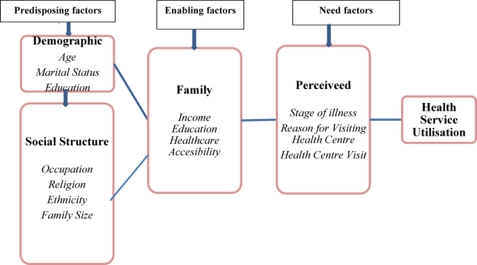
We follow a framework proposed by Anderson’s Health Behavioural model^33,34, presented in Fig. 2, which offers a robust conceptual foundation for understanding healthcare utilization by categorizing determinants into predisposing, enabling, and need factors. In the context of cancer, these determinants shape household’s decision-making process regarding whether and how to seek treatment optimally. Based on this framework, we propose a simple theoretical model (in a static framework) (see Supplementary Appendix A1) for optimal healthcare utilization in the presence (or absence) of healthcare insurance and other provisions of informal insurance (like social networks for easing healthcare accessibility, financial assistance from relatives, friends and neighbours). The static model formalizes a utility-maximizing framework, thereby offering a microeconomic insight into cancer healthcare utilization decisions under resource constraints. The out-of-pocket expenditure is the source of financing the cancer treatment in the absence of any insurance. In such a situation, the household faces severe economic hardship and may face catastrophic health expenditure and financial distress due to depletion of savings or indebtedness.

Andersen’s behavioural model of healthcare services.

The empirical exercise presented in the following section is conceived from this theoretical framework.

Propensity score matching

The economic burden of Cancer on households can be attributed in terms of healthcare utilisation and healthcare expenditure. The outcome variables for capturing the impact of healthcare utilisation include inpatient visits, length of stay in the hospital, number of surgeries, medicine uptake, diagnostic tests and outpatient visits. The outcome variables for economic burden are characterised under healthcare expenditure (includes medical expenditure, transportation expenditure and total expenditure in respective inpatient and outpatient cares), and financial hardship as well as coping strategies (include borrowing and selling of assets, and effect on income, work, and non-medical consumption) (see Table A1 and A2 in the Appendix). It is also likely that the CA households may experience induced adverse spill-over effects on the rest of the family members due to financial constraints (owing to the exorbitant OOP healthcare expenditure of the Cancer-affected member). Therefore, we explore the effect by analysing the rest of the household members’ healthcare utilisation (highlighted as non-cancer diseases (all major diseases except cancer) and non-major diseases (all diseases with the exception of cancer, diabetes, stroke, and heart disease)) and healthcare expenditure.

Since there can be multiple ailing members with multiple healthcare utilisation in a single household, we have standardised the outcome with respect to household size to make outcomes comparable between CA and NCA. We have also analysed the institutional differences in healthcare delivery between public and private healthcare. The treatment effect (of Cancer) is thus interpreted in terms of per household member (p.m). For example, ‘Inpatient visit p.m.’ implies, average inpatient visits of household members when affected by ailments.

The effect of Cancer on households in terms of healthcare utilisation, healthcare expenditure, and financial hardships (including coping strategy) is explained by the following equation:

Where \(\:Y\) denotes the outcome variables (various indicators of healthcare utilisation or economic burden) for household i, D is a dummy which is equal to 1 if any member of a household is affected by Cancer and 0 otherwise, and X is a vector of covariates that might influence the outcome. The assignment of treatment and control is not random as the CA and NCA households may differ in terms of demographic, socioeconomic, and regional characteristics and in the presence of unobservable heterogeneous Cancer risk factors. Given that the treatment (Cancer) is not likely to be random ensuring internal validation is challenging. Furthermore, health-seeking behaviour in the absence of social health security becomes self-selective in nature and is subject to the socioeconomic gradient. This may lead to potential selection bias due to the violation of OLS assumptions and may yield inconsistent estimates. In other words, the covariance of D and the error term would be non-zero (\(\:Cov\left(D,\:\epsilon\:\right)\ne\:0\:)\) if the unobservable factors influence the self-reporting of Cancer. Therefore, we propose to adopt the propensity score matching (PSM) method to estimate Eq. (1). The quasi-experimental matching technique attempts to “balance” the distribution of covariates in the treated and the control group to mimic the randomisation framework (see the Supplementary Appendix A2) for the methodological details of PSM). The advantage of PSM compared to other parametric methods is that it does not rely on any functional assumption between the treatment and outcome³⁵, and is also robust to selection bias³⁶.

The primary objective is to estimate the Average Treatment Effect on the Treated (ATT) on health outcomes between CA and NCA households by using a non-experimental secondary dataset. Thus,

Where \(\:{Y}_{1i}\) is a health outcome of a household i when any member has Cancer and \(\:{Y}_{0i}\) is what the health outcome of a CA household i would have experienced when the member is afflicted with non-cancer diseases. The parameter \(\:E\left({Y}_{1i}|{D}_{i}=1\right)\) is an average health outcome when a household is afflicted with cancer, while \(\:E\left({Y}_{0i}|{D}_{i}=1\right)\) is a counterfactual, i.e., what would have been an outcome of a CA household in the absence of Cancer (but with other ailments). However, \(\:E\left({Y}_{0i}|{D}_{i}=1\right)\:\)is unobserved, so cannot be measured. The estimator \(\:E\left({Y}_{0i}|{D}_{i}=0\right)\) can be a measurable proxy for the counterfactual, but it would lead to a biased estimates because of the inherent pre-treatment difference between CA and NCA households. In order to estimate the average treatment effect of the treated (ATT), the matching requires the unobserved \(\:E\left({Y}_{0i}|D=1\right)\) to be replaced with observed household, say t, from the control group, such that it is matched to the observation i on a vector of pre-treatment X (i.e., X_i ≈ X_t). The unmatched observations are pruned from the data set before further causal analysis. The implicit assumption is that the reporting for Cancer is conditioned on observed covariates. The PSM identifies the matched counterfactual by summarising the effect of vector X into a scalar quantity represented by conditional probability called propensity scores. It is specified as;

We predict the probability (propensity score) of a household with at least one member reporting for Cancer (CA) conditioned on X using the logit model,

The households in the treatment and control groups with similar observable characteristics in the pre-treatment are supposed to have similar propensity scores. Thus, it ensures a situation similar to a quasi-randomisation where β is a vector of parameters to be estimated for the treatment effect.

PSM requires that the mean of the respective covariates used for matching should not be statistically different for the control and the treated groups. The balancing property and area of common support assumption are checked before estimating ATT. We estimate the causal effect of cancer on households compared to other diseases using four popular propensity score matching techniques (nearest-neighborhood, radius, kernel, and stratified matching), given that each algorithm has its own advantage³⁷. The ATT measures the average treatment effect on the treated, i.e., the effect of cancer on CA households.

Regression adjusted matching

Given the negligible social health insurance coverage in India, the impact of cancer might have socio-economically heterogeneous effect on households. To check such heterogeneous effect of Cancer on households with different socioeconomic groups (based on education and social groups), we conduct a separate analysis by running a two-stage regression-adjusted matching method. To understand whether there is a significant difference in healthcare utilisation among the CA and NCA households based on the heterogeneous effect of socioeconomic status: (1) measured by educational attainment (Low Socioeconomic Status (LSES) for education below primary and (2) social groups (disadvantaged social categories in India -Scheduled Castes (SCs) and Scheduled Tribes (STs). These social categories are the historically discriminated and marginalized sections and have been therefore declared reserved categories for affirmative actions after India’s independence.

We first identify the matched counterfactuals and drop the remaining unmatched samples before applying parametric regression models. The detailed estimation process is provided in the Appendix (see section A3).

The following regression-adjusted matching equation:

Here, Y is an outcome variable, and CA is a binary indicator variable with 1 as cancer-affected household and 0 otherwise; (LSES)/(ST/SC) is a binary indicator variable with 1 being household is LSES, 0 otherwise (with 1 means household being ST/SC, 0 otherwise); and CA*LSES is an interaction term; \(\:\epsilon\:\) is an error term; \(\:\alpha\:,\beta\:,\gamma\:\:and\:\delta\:\) are the parameter of our interest. The coefficient \(\:\beta\:\) is the difference in outcome for CA and matched NCA households belonging to the non-LSES (non-ST/SC) households. The sum of coefficient \(\:\beta\:+\:\delta\:\) can be interpreted as the difference in outcome for CA households and matched NCA households for LSES (ST/SC). Thus, the test of equivalence or no difference in healthcare outcome under the Null hypothesis—H₀: \(\:\delta\:=0\), which assume that there no statistical ‘difference’ in outcomes for CA households in LSES (ST/SC) as compared to Non LSES (ST/SC) households (i.e., equality in healthcare utilisation, healthcare expenditure, and financial hardship across groups, compared to the reference group) (see Appendix: Section A3 for methodological detail).

Robustness and sensitivity analysis

The given data reports that majority of the Cancer cases are hospitalisation cases. Moreover, NSS database does not provide the cause of death in a household. If we ignore these facts, it may overestimate the effect due to possible differences in healthcare utilization and expenditure due to death during the survey round and also the risks of retaining outliers in healthcare visit and health expenditure due to end stage treatment (during the last 365 day recall period). So, we have adopted different robustness strategies to avoid such pitfall. We conducted more heterogeneity analysis through several sub-sample estimation of ATTs by (1) including hospitalisation, (2) excluding hospitalisation, (3) dropping the households reporting for the death of any member; and (4) dropping the households in top 1% of the total expenditure incurred due to Cancer (to avoid potential upward bias in the impact of Cancer on households), and then estimating ATT using the scores respectively. We conducted couple of subgroups analysis separately for possible heterogeneous effect of Cancer on the disadvantaged households by taking education (household head with primary or below primary education level.

In a quasi-experimental framework, the assumption of conditional mean independence would be violated if there are unobservable factors affecting the assignment of treatment and control simultaneously, thereby leading to biased estimations. Therefore, it is important to check the sensitivity of the estimated result with respect to deviation from the identified assumption. We conduct a sensitivity analysis on PSM-based estimates to determine the potential bias due to the presence of unobservable. In Rosenbaum’s sensitivity framework, the parameter \(\:\left({\Gamma\:}\right)\) is introduced to quantify the strength of potential unobserved confounders, representing the extent to which the study’s conclusions might be influenced by factors not accounted for in the observed data³⁸.