Multidisciplinary cancer disease classification using adaptive FL in healthcare industry 5.0

In this Proposed Intelligent System for Multidisciplinary Cancer Disease Prediction, It presents how adaptive federated learning is used in the suggested intelligent system for transdisciplinary cancer illness prediction in the healthcare industry 5.0. In Fig. 1, the suggested model is shown. The stages of the suggested Intelligent System with an adaptive federated machine learning model for smart healthcare system-based multidisciplinary cancer patient prediction are as follows:

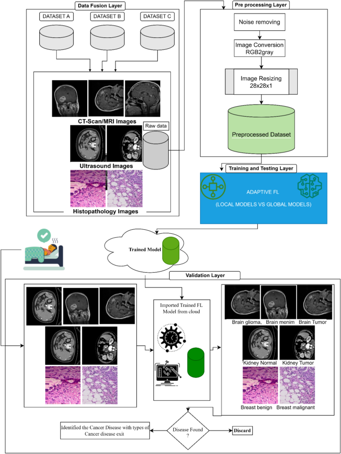
Proposed adaptive federated machine learning Model.

The proposed model is divided into four (04) phases; (1) Data fusion Layer, (2) Preprocessing Layer, (3) Training and Testing Layer, and (4) Validation Layer. In the first phase of the proposed model, we have considered the three datasets of cancer diseases named (i) brain cancer, (ii) kidney cancer, and (iii) breast cancer. The brain cancer dataset is further divided into three subtypes of cancer disease. The kidney cancer dataset has two subtypes and the breast cancer dataset also has two subtypes. All the datasets comprised 35,000 images and 5000 images in each class. The detail is shown in Table 1.

In the preprocessing layer, the fused dataset is being processed for further use in disease classification in the proposed intelligent system. A collection of procedures and techniques used on digital images before additional processing or analysis is referred to as image preprocessing. Enhancing the image’s quality is the main objective of image preprocessing, as it facilitates the extraction of valuable information by algorithms. Various methods can be applied singly or in combination, based on the particular demands of the image processing assignment. The quality and usefulness of the image for additional analysis can be significantly increased by using the necessary techniques, producing more accurate and trustworthy results.

In 2nd step, we converted all the images from RGB to grayscale to minimize the computation cost. In 3rd step, we resized the images and made the complete fused dataset smooth for further training and training of this dataset. Due to the image’s dataset, the computation cost increases with the increase of images. In our experimentation, we have considered the image size 28*28*1 for fast feature extraction and internal calculations. After completing these three (03) steps in preprocessing layers, the fused dataset is ready for experimentation. In the training and testing layer, a federated learning methodology is adopted for training and testing the dataset of multidisciplinary cancer disease classification. In our proposed adaptive federated learning, the datasets are trained as per the federated learning methodology as discussed in section “Introduction”. All the local models’ weights are exchanged with a global model for synchronization and making the accuracy level equal to each local model as per the global model. In this proposed adaptive federated learning approach, we considered three hospitals having two (02) devices installed, in each hospital, for collecting the data on each cancer disease. The dataset of each smart hospital is distributed for the training and testing model.

The detail of working and mathematical demonstration³⁹ is as under and used notation is shown in Table 2.

Consider the set \(\mathcalH = \left\ 1, \ldots ,\text N \right\\) of hospitals, and for each hospital i, we have a corresponding error function \(G_i \left( \varvecu \right)\), where \(\varvecu\) is the model vector having dimensions \(\delta , \varvecu \in R^\delta \). The optimization problem is constructed as follows³⁹,

where ‘H’ represents the number of hospitals. We want to find the u that minimizes the above equation. All of the hospitals have their own set of devices \(\mathcalH_D \left( i \right)\) such that \(i \in \mathcalH_D\) and \(\left| \mathcalH_D \right|\) is the number of devices. Next, we define a new dataset \(E_i \) as \(E_i = \left\ \varvecx,\varvecy \right\_i \) for the ith hospital where \(\varvecx\) are the measurements and \(\varvecy \) are the labels. We now assume as follows.

All devices of the ith hospital can access the entire dataset Ei of that respective hospital.

We have to partition \(E_i\) into \(H_D \left( i \right)\) smaller subsets, \(E_i = \left\{ {\left\ \varvecx_1 ,\varvecy_1 \right\, \ldots , \left\{ {\varvecx_\mathbfH_\mathbfj , \varvecy_{{\mathbfH_\mathbfj }} } \right\}} \right\}\) with the constraint that \(\bigcap\limits_k = 1^{\textH_\textj } e_k = \emptyset \) such that \(e_k \in E_i\), in simpler words, all partitions are disjoint there exists no common element between them. This is done to deal with the decentralized framework.

A model \(\varvecu\) is received by the devices from the hospital and is updated using a Stochastic Gradient Descent (SGD) optimization algorithm, the learning rate & the number of epochs for every single device are the same.

The updated model is denoted as \(\varvecu_\varvecj\) for the jth device. The error of the jth model for the kth subset of the dataset is defined as \(l_jk \triangleq l\left( \varvecu_\varvecj ;e_k \right)\) where \(e_k \in E_i\).

Next, we define the mean loss of our model over the entire dataset for the ith hospital as

The loss of each subset is calculated and summed for the given model j.

Now we can define our original \(G_i \left( \varvecu \right)\) as the sum of individual losses \(l_j\). Then the loss for the ith hospital is

For the ith hospital, the loss is the average of all the losses for \(H_D\) devices in the hospital. \(l_j\) as mentioned before is the loss of the jth model for the ith hospital.

Now we write our problem in terms of minimizing all the loss functions \(G_i\) individually, where we find the model \(\varvecu_\varvecj\) which minimizes the loss function. We now focus on the subsets instead of minimizing the sum of losses, this problem is handled as the primal assignment problem.

At the end of the training and testing process, the generalized adaptive global model of the proposed intelligent system is uploaded to the cloud for validation purposes. In the last phase of the proposed model, a validation layer is presented for the validation of new patients’ data on the trained adaptive model. In this layer, data is received from smart devices on run time, sent to a raw database, and preprocessed. After preprocessing, preprocessed image data is sent to a trained adaptive model for the classification of multidisciplinary cancer disease. If a multidisciplinary cancer disease exists, our proposed intelligent system will prompt with the label of a class of cancer disease in the patient’s body and recommend the patient to consult with a specialized doctor, else it will discarded.

A bipartite graph can be used to represent the relationship between hospitals and medical devices, where one set of vertices represents the hospitals and the other set represents the medical devices. An edge between a hospital vertex and a device vertex would indicate that the hospital has acquired or is using that device. The specific purpose of using a bipartite graph in this context is to analyze and optimize the allocation of medical devices to hospitals.

By representing the hospitals and devices as separate sets of vertices and using edges to represent their relationships as shown in Fig. 2, we can easily identify which devices are being used by which hospitals, and which hospitals have unmet device needs.

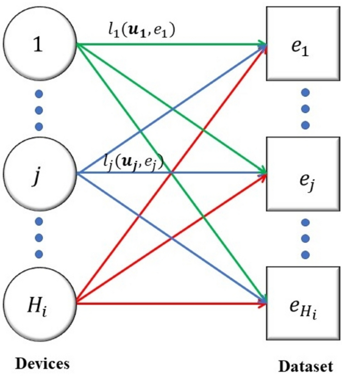
Dataset allocation of smart hospital i.

By using a bipartite graph, we can distribute the whole dataset into subsets as per the number of devices across all hospitals. This can help healthcare systems optimize their device allocation strategies to ensure that devices are being used efficiently and effectively.

Consider a bipartite graph \(\mathcalG_i^a = \left\ H_D \left( i \right), E_i ;Q_i^a \right\\) where \(Q_i^a\) is the complete set of edges and the edge \(\left( j,k \right) \in Q_i^a\) occurs if & only if, jth smart device can be allocated to the kth subset as shown in Fig. 2. We introduce a binary decision variable \(d_jk \in \left\ 0,1 \right\\) for each edge \(\left( j,k \right)\), which associates the kth subset to the jth device. The device is assigned to the subset of the variable that takes on the value of 1 and it is not assigned if it takes on the value of 0.

Now we model the problem as a multi-assignment problem

Subject to

where \(\varvecd = \left[ d_11 ,d_12 , \ldots , d_H_D \left( i \right), H_D \left( i \right) \right]^T \) is the vector of resulting variables. Similarly, the limitations illustrated that every device is to be allocated to a subset & this subset is to be allocated to a device.

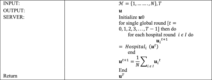
Algorithm 1: Centralized server.

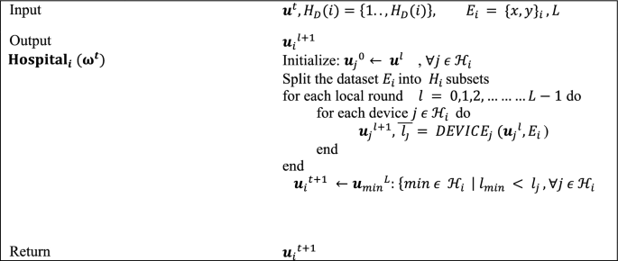
Algorithm 2: Smart hospitals.

Assume \(G_i^a\) is complete. Also, note that \(H_D^2 \left( i \right) = \left| Q_i^a \right|\) and \(d_i = H_D \left( i \right)\).

The issue is written in matrix form, succeeding the normal linear programming arrangement:

Focus to \( A\varvecd = \varvecb\).

Where \(\mathcalL \in \mathbbR^H_D^2 \left( i \right)\) denotes the losses vector \(\mathcalL = \left[ l_11 ,l_12 , \ldots , l_H_D \left( i \right)H_D \left( i \right) \right]^T\), and \(\varvecd \in \mathbbR^H_D^2 \left( i \right)\) the vector of decision variables. \(A \in \mathbbR^d_i \times H_D^2 \left( i \right)\) are the limitations of matrix and \(\varvecb = \mathbbR^d_i \) is a vector of ones.

The network of \(H_D \left( i \right)\) devices of the hospital i are modeled by a directed graph (digraph) \(\mathcalG_i^c = \left( \mathcalH_i ,Q_i^c \right).\) \(\mathcalH_i\) is the set of devices and \(Q_i^c\) is the set of edges such that it is a subset of the Cartesian product of \(H_D \left( i \right)\), \(Q_i^c \subseteq H_D \left( i \right) \times H_D \left( i \right)\), where \(\left( j,k \right) \in Q_i^a\) if the nearby edge moves from j to devise k.

In the first Algorithm, the vector W₀ of the model is arbitrarily prepared and delivered to each hospital, beginning with the centralized server. The numeral of the universal aggregation round is denoted by T. When the model arrives at the hospital, the local training phase begins, as indicated in the smart health Algorithm. When the local training of the model is finished, the hospital chooses the local model with minimum loss and transfers it to a centralized server for universal aggregation. During this step, every single model is evaluated, and only the one that has the best performance on the entire dataset is forwarded to the centralized server.

Each smart hospital organizes the local training operation in Algorithm 2 by adjusting the accessible hospitals’ devices and it also splits the image dataset. The numeral of local training cycles is L, the number of devices is H_D (i), and the hospital dataset is Ei. During universal round t, hospital i obtains the universal Wt model from the central server and uses it to initialize the local model wj0 of each device j. The hospital distributes the model to each device before the first local round and allows permission to the complete segregated dataset Ei.

Following that, the hospital collects the updated local model wjl+1 as well as the related average loss j. Lastly, following the last local round of each hospital, each hospital returns the model having the lowest loss to the server.

In the third Algorithm, each device generates its loss vector Lj, the entries of which correspond to the estimated losses of model wlj on each subset. The initialization of the Decentralized Optimization function is done with Lj and Ei. In federated learning, decentralized optimization entails jointly training a global model on several decentralized devices without sharing raw data. First, a global model is transmitted to the participating devices after being set up on a central server. After that, each device trains the model independently using its local data, calculating gradients that indicate parameter changes for better results. To maintain privacy, only these gradients are sent back to the central server as opposed to raw data. These gradients are combined by the central server, which then modifies the global model. Until convergence, this repetitive sequence of global model update, communication, aggregation, gradient computation, and local training is repeated. By utilizing a decentralized method, devices can overcome privacy concerns in collaborative machine learning by improving models while maintaining localized data. The function handles the multi-assignment problem by executing the Distributed Simplex algorithm⁴⁰. α is a scalar that reflects the assignment problem solution; in other words, it determines which subset of the dataset will be trained in the upcoming local cycle.

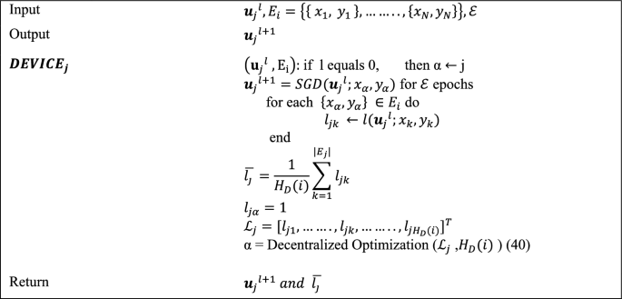
Algorithm 3: Smart hospital device.

The initial local cycle is started with the value j, which corresponds to the device numeral, such that all the devices train their models at subset j of the dataset. In this technique, an updated model \(\varvecw_j^l + 1 = \varvecw_j^l – \eta \nabla l\left( w_j^l ;x_\alpha ,y_\alpha \right)\) is computed on the subset chosen by using the Stochastic Gradient Descent⁴¹. E denotes the numeral of epochs, and \(\eta\) represents the learning rate of the model. We reprimand the conclusion to train the model in the earlier selected subset before the next local round by assigning the extreme value ‘1’ to the loss j, which resembles the preceding choice.

The application of Convolutional Neural Networks (CNNs) is essential for improving the precision and effectiveness of cancer categorization. In particular, CNNs are essential for the interpretation of complex medical images from a variety of sources, including histology slides, CT scans, and MRIs. They are skilled at recognizing patterns suggestive of various cancer kinds because of their capacity to automatically extract hierarchical features. CNNs can be installed throughout dispersed healthcare facilities in the framework of Adaptive Federated Learning, facilitating cooperative model training without requiring the exchange of private patient information. This decentralized method complies with healthcare confidentiality regulations. The integration of CNNs into this multidisciplinary framework for classifying cancer diseases within Healthcare Industry 5.0 demonstrates the dedication to utilizing cutting-edge technology for accurate and customized cancer diagnosis, ultimately leading to better patient outcomes.

A thorough case study can shed light on how this strategy is used in real-world healthcare situations and how beneficial it is. The graphical representation of the proposed model hierarchy between different layers is shown in Fig. 3. Local optimization is carried out in the layer of smart devices, and the suggested model is trained and displayed in Fig. 3 of the Convolutional Neural Network (CNN). The goal of the communication between all of these levels is to create a generalized adaptive federated learning model. To create a new master model, the weights of all the local models are shared with the global model. This approach continues until the global model and the learning criteria are the same. Finally, for testing and validation, we provided the cloud server with the generalized global model. The main advantage of using CNNs in federated learning is their ability to learn complex representations from raw input data, making them well-suited for tasks such as image recognition. Additionally, CNNs are relatively lightweight and can be trained efficiently on mobile devices, making them well-suited for federated learning scenarios. To support the suggested model’s functionality, we used reputable datasets for the multidisciplinary classification of cancer diseases in this study as a case study. Three datasets are combined to provide the simulation and findings.

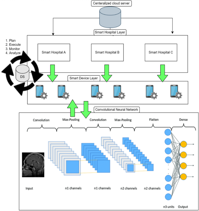
Graphical representation of flow chart hierarchy of proposed model.

Dataset

We used multiple cancer datasets³⁸, containing eight (08) types of cancer image datasets. We considered only three cancer diseases in our case study; (1) brain cancer, (2) breast cancer, and (3) kidney cancer. Brain cancer is divided into three sub-folders of different types of brain cancer. All these subfolders contain a total of 15,000 images and 5000 images in each class of cancer. Breast cancer and kidney cancer have two subclasses. Both these datasets are comprised of 20,000 images and each dataset has a 10,000 images dataset. The data fusion approach is used for making an enriched dataset for the classification of deadly multidisciplinary cancer diseases. This fused dataset contained 35,000 images of seven (07) subtypes of cancers. The experimentation and classification of cancer are done through an adaptive federated learning approach empowered with CNN as discuss above.